Published in Synthetic Information October 8, 2013
Updated JULY 18, 2014
Updated August 10, 2014
Updated October 10, 2014
Updated November 28, 2014
Updated March 24, 2015
"Science is the belief in the ignorance of the experts."
- Richard P. Feynman
"Rational skepticism is the foundation of Science."
- Any real scientist
Climate change is inevitable.
-The Management
Statistical inference is the enemy of causality.
- The Management
WSJ: http://tinyurl.com/laszrkuUpdated JULY 18, 2014
Updated August 10, 2014
Updated October 10, 2014
Updated November 28, 2014
Updated March 24, 2015
"Science is the belief in the ignorance of the experts."
- Richard P. Feynman
"Rational skepticism is the foundation of Science."
- Any real scientist
Climate change is inevitable.
-The Management
Statistical inference is the enemy of causality.
- The Management
We are very far from the knowledge needed to make good climate policy, writes leading scientist Steven E. Koonin
Leading American Scientist Steven E. Koonin writes about fundamental problems inherent to Climate Models. Echos criticism of Climate Models we have identified for some years in this blog.
The fact that IPCC climate models have failed to accurately forecast the climate is a huge problem for the credibility of Climate Science.
Over the years we have predicted on theoretical grounds that non-causal climate models, such as the IPCC models, would inevitably fail when extrapolated into the future. Specifically, we outlined weaknesses in the methodology of climate modeling that lead to such failures.
See below previous posts for reference:
______________________________________
Why Must Climate Models Fail on Extrapolation?
http://syntheticinformation.blogspot.com/2013/05/why-climate-models-fail-at-extrapolation.html
Published in Synthetic Information May 11, 2013
http://syntheticinformation.blogspot.com/2013/10/why-is-global-averaged-temperature-anon.html
Published in Synthetic Information October 8, 2013
What is Modeling?
http://syntheticinformation.blogspot.com/2011/07/what-is-modeling.html
Published in Synthetic Information July 5, 2011
______________________________________________________________________
ABSTRACT and INTRO
In the hard sciences such as physics, physical theories like Newtonian mechanics, Maxwell's electrodynamics, Einstein's General Relativity, Quantum Mechanics, Quantum Electrodynamics, and the Weinberg-Salam-Glashow Electro-Weak Interaction Theory, to mention a few, have secure, and rather rigorous mathematical formulations, and are capable of making predictions which agree with best highly sophisticated experimental tests, within their energy ranges of validity. That is, the above theories have been tested by rigorous, repeatable, controlled experiments over many trials, over many years.
Scientists Use the Scientific Method:
What's That?
This procedure of testing predictions of theory by experiments, so as to provide rigorous re-confirmation of predictive accuracy, is known as the scientific method. The scientific method is the means of progress in the natural sciences. If you are not using the scientific method, you are not doing science.
"Extraordinary claims, as the saying almost goes, demand more scrutiny than usual to make sure they stand up. That is how science works. Claim and counter-claim: intellectual thrust and experimental parry." REF: Nature October 14, 2014
SIDE BAR
The scientific method applied to climate models
In order to apply the scientific method to climate models, we must identify the hypothesis being tested when we compare climate observations with the predictions of climate models. Not as easy as it sounds.
Hypothesis:
Existing climate models can be used to forecast the climate accurately.
Scientific Test Procedure for climate models:
Step 1
Obtain climate model predictions for the evolution of climate observables over some future time interval.
Step 2
Wait around while observers (experimentalists) collect accurate data over the time interval. (assumes observers use accurate calibrated monitors for the quantities being measured, and that they don't fudge the data)
Step 3
Compare data collected
(values obtained for measured observables during the time interval of interest)
to predicted values of those observables over the same time interval.
Step 4
If the comparison shows the model's prediction deviated significantly from the observed data over the time interval, the climate model being tested is invalidated. Hence, the hypothesis:
"Climate models can accurately forecast the climate (over the stated time interval)"
would be disproved.
Notice that the hypothesis we can test is not this:
"Does human activity cause future global warming?"
Instead it's this:
"Did the climate model being tested accurately predict the future of the climate (as claimed by its proponents) or not?"
If a climate model prediction is contraindicated by the data, the model is considered invalidated, and the hypothesis is disproved.
Back to climate theory and climate models...
In clear distinction to physical systems described so accurately by the above theories from physics, the earth's climate has no such rigorous testable theory. Why is that? Good question.
Part of the Answer:
Unlike the above mentioned physical theories, controlled experiments are not available to test climate theories. Why not? Well, we do not have sufficient control over the enormous collection of variables required to determine the state of the earth's climate. This limits or precludes controlled repeatable experiments of the sort needed to test climate theories. Simply put, controlled experiments cannot be done on the earth's climate.
The Other Part of the Answer:
We scientists do not have a rigorous causal theory of the earth's climate. More on causality in physical theories later.
What?? You mean we have no way to test a global climate theory, even if we had a global climate theory, which we don't? Yeah, that's exactly what I mean. Deal with it.
Ok, given that we don't have controlled climate experiments, nor a rigorous causal climate theory, what do we have instead? Well, we have climate models.
Climate Models
Right. So what are climate models? Read on.
Models of the sort used by the climate modelers play a rather minor role in the hard sciences. That's why you don't hear much about models or modeling in the hard sciences. Modeling is generally viewed as a low level activity mainly useful for analysis of experimental data. It comes as no surprise to scientists that climate models are so often wrong, and so often modified.
In this paper, we examine modeling, its inherent flaws, assumptions, and limitations.
Further, we identify a few commonly encountered misapplications of climate modeling as currently practiced.
Further, we identify a few commonly encountered misapplications of climate modeling as currently practiced.
Central Problem, a Question and Discussion
Perhaps the central problem with climate models is that they do not obey physical causality.What is meant by the term physical causality? Why is it bad for a model or theory to disobey it?
Read on for more on these questions, but first:
We ask the question:
Is the methodology of climate modeling fundamentally unsound?
Further, we examine the track record of climate forecasting models. Over the past two decades substantial new climate data has become available from accurate sophisticated monitoring and imaging systems. We will highlight global sea ice measurements made by modern satellite imaging systems.
Importantly, these new data were acquired after climate modelers made their predictions about sea ice. More generally, climate forecasting models are now subject to a host of new critical tests. Did their widely publicized predictions come true? How badly have climate model forecasts missed the mark?
In science, if model disagrees with new data in any significant way, that is, if a model forecast or prediction is contraindicated by new data, the model is invalid, or just plain wrong. Maybe the model can be fixed up, and maybe not. When model predictions exhibit significant long term divergence from new data, it's a strong indication that the underlying methodology of the model is fundamentally unsound. That's how the scientific method works for models of observable quantities.
In scientific modeling, new models are always suspect. Old models can be valid, but only if they are validated by new data. Further, valid old models that diverge from new data become invalid old models. The scientific method requires rather stringent conditions be met by models, and models are happily discarded if they don't make the grade. If something is learned from the erroneous model, we have scientific progress.
In climate modeling, new models are bad unless proved good by experiment. That is, new models have no scientific standing or claim to validity until validated by actual observed agreement with future data. The graveyards of science are filled by new models that subsequently failed to pass rigorous testing and repeated confirmation by experiments.
Should the Lemon Law Apply to Climate Models?
When climate models are churned out annually, biannually, or multiannually, newly tweeked to fit the latest data, as new models, they have no validity. Model validity is only acquired if predictive accuracy is demonstrated over many future years, without further tweaking. Models that undergo periodic tweaking to agree with new data become little more than curve fitting exercises, no matter how fancy the graphics. This kind of ad hoc methodology amounts to little more than pure empiricism.In science, old models may be valid or invalid. New models are always invalid (or unvalidated) until tested. They may become validated after they demonstrate substantial agreement with new data (i.e. data collected after the release date of the model in question.)
Climate modelers are in an embarrassing situation. Searching questions about the validity of the climate modeling industry are being asked. Is the climate modeling process fundamentally flawed? Is climate modeling a lemon?
When we purchase a new car that breaks down, and is generally unreliable during the next year after purchase or repair, the car is considered a lemon and can't be fixed. We have legal grounds to return the car to the manufacturer and get our money back.
If a pharmaceutical company comes up with a new drug, how do we consumers know it's effective and safe? We don't, nor does anyone else know. We only find out by clinical trials over many months or years that confirm effectiveness and safety.
Like new untested drugs, new climate models should be considered unusable until thoroughly tested and proved effective over time. If we hold climate models to this clinical standard, well...the old models didn't make it through clinical testing, and new ad hoc models probably won't either.
For climate models, a miss (systematic divergence from new data) is as good as a mile (total invalidation.)
Our broker would say: It's probably time to sell climate modeling short. Take the loss, and get out of that position.
BACKGROUND: Extravagant Claims of Predictive Accuracy
Recall that the proponents of climate models themselves made repeated extravagant claims of the predictive accuracy of their models. Extravagant claims of predictive accuracy must be backed up by extraordinary agreement with future data. For the climate modelers, a miss is as good as a mile.
Misapplication of models has given the process of modeling a bit of a shady reputation in scientific circles. Long term systematic disagreement with new data might be an indication that a critical piece of the physics of the system is not included in the model. However, in modeling, long term systematic disagreement with new data is often the result of a much deeper problem. Stated in a formal way, long term systematic disagreement with new data can be a consequence of fundamentally unsound methodology inherent in the process of modeling.
An example of sketchy methodology used in climate modeling is the use of proxy time in animations.
How is proxy time used?
Many climate models make use of an artificial time variable, sometimes called proxy time.
Proxy time is used like this: A sequence of static images are attached to an artificial time variable. When the sequence of images are played back, one has what appears to be a time dependent animation.
Why is this is a risky procedure?
It's risky and misleading because the real time dependence of the system being modeled need not follow the animation. Such models do not obey strict causality (they are non-causal models) even though they may be made to appear causal when animated using proxy time.
Proxy time animations generate pretty pictures that have no causal interrelationship. That's dangerous and (often) misleading to the viewer. Such animations need not follow the actual time evolution of the real physical system being modeled. They give a fake future of the system being modeled.
Animations of an anvil falling on the Coyote do not accurately simulate a real anvil falling on a real Coyote.
Climate model animations using proxy time might appropriately be called Climatoons or Proxytimeatoons.
Proxy time Climatoons are not educational, cool, cute, or funny. They are misleading to the uninformed, and of little scientific value.
Don't be fooled by Climatoons.
In the following, we observe that non-causal models of complex systems inevitably fail on sufficiently long time scales.
What is Global Average Temperature?
Real Scientists know this about GAT:
Global Average Temperature is not a measure of the heat content of the Earth's atmosphere. Nor is it a valid thermodynamic quantity. It turns out that changes in Global Average Temperature do not tell us how much heating or cooling is occurring in the atmosphere.
Here's why.
(A bit technical, but here is a brief description of the difficulty.)
The Earth's atmosphere is not in a state of thermodynamic equilibrium, hence the rigorous physical theory of heat, Thermodynamics, does not apply to the Earth's atmosphere. This means that Thermodynamic formulas cannot be applied to the atmosphere as a whole. Hence there is no rigorous theory of the heat content of the atmosphere as a whole.
Instead of thermodynamics what do we have?
In order to make progress, fluid theory makes use of an assumption called local thermodynamic equilibrium (LTE). LTE is not a bad approximation in much of the atmosphere, but not so good at high altitudes. Most physicists would be inclined to accept the validity of LTE in the atmosphere and perhaps rely on fluid transport equations for modeling purposes. However, there is a non-trivial difficulty in the fluid equation approach in the case of earth's atmosphere.
In LTE systems thermodynamics is valid locally, (in small volumes of gas inwhich the temperature is constant throughout), the amount of heat in such a small volume of atmospheric gas is not given solely by the local temperature.
Instead, one needs the local temperature and a quantity known as the local specific heat of the atmospheric gas. The product of local temperature, gas density, and local specific heat yields a measure of the total heat content of a small local volume of the atmosphere.
However, we don't really measure the heat content of the Earth's atmosphere, nor do we know it as a function of time.
The heat content of a local sample of the atmosphere is dependent on the local specific heat per particle, on the local composition of gas species in the atmosphere, and on many other variables including the local composition of clouds, water vapor, dust, and the like.
This presents a problem for climate models. The values of this local specific heat, and local atmospheric composition are not known (measured) throughout the real atmosphere of the Earth. The local heat content depends on many variables, not all of which are measured or known accurately everywhere in the atmosphere.
More on this later, as space permits...
In a recent piece in Nature, climate modeling was caricatured as educated guesswork combined with fancy graphics.
What is Global Average Temperature?
Real Scientists know this about GAT:
Global Average Temperature is not a measure of the heat content of the Earth's atmosphere. Nor is it a valid thermodynamic quantity. It turns out that changes in Global Average Temperature do not tell us how much heating or cooling is occurring in the atmosphere.
Here's why.
(A bit technical, but here is a brief description of the difficulty.)
The Earth's atmosphere is not in a state of thermodynamic equilibrium, hence the rigorous physical theory of heat, Thermodynamics, does not apply to the Earth's atmosphere. This means that Thermodynamic formulas cannot be applied to the atmosphere as a whole. Hence there is no rigorous theory of the heat content of the atmosphere as a whole.
Instead of thermodynamics what do we have?
In order to make progress, fluid theory makes use of an assumption called local thermodynamic equilibrium (LTE). LTE is not a bad approximation in much of the atmosphere, but not so good at high altitudes. Most physicists would be inclined to accept the validity of LTE in the atmosphere and perhaps rely on fluid transport equations for modeling purposes. However, there is a non-trivial difficulty in the fluid equation approach in the case of earth's atmosphere.
In LTE systems thermodynamics is valid locally, (in small volumes of gas inwhich the temperature is constant throughout), the amount of heat in such a small volume of atmospheric gas is not given solely by the local temperature.
Instead, one needs the local temperature and a quantity known as the local specific heat of the atmospheric gas. The product of local temperature, gas density, and local specific heat yields a measure of the total heat content of a small local volume of the atmosphere.
However, we don't really measure the heat content of the Earth's atmosphere, nor do we know it as a function of time.
The heat content of a local sample of the atmosphere is dependent on the local specific heat per particle, on the local composition of gas species in the atmosphere, and on many other variables including the local composition of clouds, water vapor, dust, and the like.
This presents a problem for climate models. The values of this local specific heat, and local atmospheric composition are not known (measured) throughout the real atmosphere of the Earth. The local heat content depends on many variables, not all of which are measured or known accurately everywhere in the atmosphere.
More on this later, as space permits...
The Fallacy of Proxy Time
Fallacy: noun- a mistaken belief, especially one based on unsound argument."the notion that the camera never lies is a fallacy"
synonyms: misconception, misbelief, delusion, mistaken impression, error, misapprehension,misinterpretation,
misconstruction, mistake
An example of sketchy methodology used in climate modeling is the use of proxy time in animations.
How is proxy time used?
Many climate models make use of an artificial time variable, sometimes called proxy time.
Proxy time is used like this: A sequence of static images are attached to an artificial time variable. When the sequence of images are played back, one has what appears to be a time dependent animation.
Why is this is a risky procedure?
It's risky and misleading because the real time dependence of the system being modeled need not follow the animation. Such models do not obey strict causality (they are non-causal models) even though they may be made to appear causal when animated using proxy time.
Proxy time animations generate pretty pictures that have no causal interrelationship. That's dangerous and (often) misleading to the viewer. Such animations need not follow the actual time evolution of the real physical system being modeled. They give a fake future of the system being modeled.
Animations of an anvil falling on the Coyote do not accurately simulate a real anvil falling on a real Coyote.
Climate model animations using proxy time might appropriately be called Climatoons or Proxytimeatoons.
Proxy time Climatoons are not educational, cool, cute, or funny. They are misleading to the uninformed, and of little scientific value.
Don't be fooled by Climatoons.
Climate Models and Climate Forecasting
In the following we observe that climate models used and misused to predict the future are more accurately termed climate forecasting models. Climate forecasting models get no credit for predicting the past. Agreement with past data is no guarantee of future predictive accuracy.
Recall that vocal proponents of climate forecasting models, themselves, have made repeated extravagant claims of predictive accuracy. We might say those proponents are guilty of repeated extravagant claim making. How good is the track record of climate forecasting models? Now we can find out.
Over the past few decades substantial new climate data has been accumulated using sophisticated monitoring and imaging technology. This new and extensive climate data present more rigorous tests of the widely announced predictions of climate models. It is now clear that new climate data accumulated 1995-2013, when compared to predictions of pre-1995 climate models show that those models have often (nearly always) diverged significantly from the real climate.
In the following, we compare a few egregious climate model predictions to new data, and explain our view that the methodology used in climate models is inherently flawed.
We observe that non-causal models of complex systems inevitably fail on sufficiently long time scales. This kind of failure is a consequence of flawed methodology, and can't be fixed.
Climate forecasting models and their failures.
Recall that in the 1990s many IPCC Climate models predicted a steady year-on-year reduction of north polar sea ice. Some models even predicted the north polar ice cap would melt entirely by 2013. These climate model predictions received so much publicity over the decades, that (probably) no reference source is needed. Remember the sad polar bears on floating ice blocks?
SIDE BAR
What about sea level rise?
What about sea level rise?
If all the sea ice melts how much will sea level rise? Answer: Zero.
Why is that? As is well known since antiquity, Archimedes' principle of buoyancy can be formulated as: The amount of water displaced by a floating object is equal to the weight of the floating object. Ice floats because its density is lower than that of liquid water. So, when a floating block of sea ice melts, and turns into a liquid, it exactly fills in the space displaced by the solid block before it melted. No change in sea level.
Here's the latest data, and it's really impressive.
Since 2005 substantial new detailed data on arctic sea ice coverage has been collected using sophisticated satellite imaging technology.
For example, we now have excellent data on sea ice coverage from the Ocean and Sea Ice, Satellite Application Facility (OSISAF).
Typical of this satellite data is the graph below from DMI Centre for Ocean and Ice for the daily ice coverage plotted for each of the years to date 2005-2013.

REF: This data and graph from DMI Center for Ocean and Ice
FIG. 1: The above figure is a copy of a figure published by DMI Center for Ocean and Ice. They caution that the absolute calibration of the area coverage may be a bit uncertain. That is, the y-axis tic marks may be uncertain by a proportional scale factor. However, the relative accuracy year-on-year is good. Click the link above for the original graphic on their website and more on these details.
What data is plotted in this graph?
Fig. 1 shows detailed data on seasonal variations (from January 1 through December 31) of sea ice area (in units of millions of square kilometers,) for the years 2005 through 2012, and January to date (mid-October) of 2013. Data for each year is color coded by the legend at the lower left of Fig.1. The black curve displays the most recent data from the current year, 2013.
Some observations on these data:
First, the maximum north polar sea ice coverage occurs in the month of March, and the maximum area of coverage ranges from roughly 10.5 to 11.5 million km^2. The minimum sea ice coverage occurs in the month of September, and the minimum sea ice coverage area ranges from roughly 2.5 to 4.3 million km^2. Every year the sea ice area cycles between these maxima and minima in March and September.
Second, we observe that the north polar sea ice coverage over 2013 (black curve) is generally higher or comparable to the average of years 2005 through 2012.
Third, in the month of October 2013 the measured arctic sea ice extent is relatively larger than all previous year's October coverage. That is, arctic sea ice reached record high levels in October 2013, according to month-on-month comparisons over available data from previous years (2005-2012.)
Fourth, in the year 2013 there is plenty of north polar sea ice in existence, comparable to previous years. The polar ice cap did not completely melt down, nor cease to exist.
What can be said about the accuracy of IPCC climate model predictions?
First, it is clear that many of the highly publicized IPCC climate model predictions about polar ice cap meltdown or steady year-on-year sea ice reductions did not occur.
Second, but most importantly, we can say that many IPCC models are contraindicated by this new data. When model predictions fail to match new data in any significant way, the model is invalidated. Hence those IPCC models are proved to be invalid by data from the field.
Can those models be fixed up? We doubt it. We observe that non-causal models of complex systems inevitably fail on sufficiently long time scales. This kind of failure as a consequence of flawed methodology, and can't be fixed.
Of course, models can be tweeked, modified or otherwise fixed up after they fail. When modelers do this in a way that agrees with the latest data, we have a new model. After such ad hoc fixes, the new models are considered invalid until they demonstrate significant long term agreement with new data, without further tweeking.
More on proxy time:
The parameter representing time, the time variable, does not appear in the physical theory of thermodynamics. One has thermodynamic state variables, but no time variable. Further, many climate simulation models do not support a time variable at all. For example, steady state flow models of the earth's ocean and atmosphere solve a set of equilibrium equations (with boundary) that do not have time as a variable.
How can such models having no time variable, be used to predict the future time evolution of the system?
Many such models make use of an artificial time or proxy time. Some quantity that varies monotonically with time, is used as a substitute for the time variable.
For, example, during time periods where atmospheric CO2 concentration is increasing steadily (monotonically) with time, one can plot model output as a function of CO2 concentration. Some modelers convert the independent variable from CO2 concentration to a proxy time variable in order to plot the model output as a function of proxy time.
Successful Non-causal Models Exist and are Especially Useful for Describing Periodic Phenomena.
Interestingly some non-causal models can exhibit excellent long term predictive capabilities in a restricted range of model parameters for simple systems. For example, Newtonian gravitational field theory coupled with classical Newtonian mechanics is a non-causal model.
Why do we say Newtonian gravity is non-causal?
The Newtonian gravitational field equations are non-causal because they exhibit instantaneous action at a distance. There are no gravitational waves or propagation speeds for changes in the Newtonian gravitational field. General relativity on the other hand, does exhibit causality, there is no "action a a distance" in general relativity. Changes in the metric propagate at the speed of light in general relativity.
SIDEBAR
Back to Newtonian Mechanics...
Further, Newtonian mechanics does not obey the rules of special relativity. Despite these problems, Newtonian mechanics can work quite well as a predictive theory.
For simple systems, e.g. planetary orbits and the like, standard Newtonian gravity and mechanics have excellent predictive capabilities and often show impressive long term agreement with measured motions of planets, asteroids, some comets, slow speed space ships, etc. In many cases, the agreement with new measurements (data) extends over many years and many orbital periods. Importantly, periodic or quasi-periodic phenomena are often well described by non-causal models.
But Newtonian mechanics does not always work. The theory is contraindicated by measurements of time evolution of the perihelion of the planet Mercury. Further, Newtonian mechanics does not work for objects having velocities approaching the speed of light. Nor does Newtonian mechanics predict the observed deflection of light by massive objects (gravitational lens effect.) Enough on Newtonian mechanics for now.

Fig. 2 Southern Hemisphere Sea Ice Area, Seasonal Variation by Year.
This data from agencies NOAA, NSIDC, and University of Bremen. Original data plot from this site: http://arctic.atmos.uiuc.edu/cryosphere/arctic.sea.ice.interactive.html
Briefly, the extensive data in this composite plot shows seasonal variations in southern hemisphere sea ice extent over 34 years from 1979 through 2013. We observe that record high sea ice extent occurred in 2013 yellow curve, and in 2012, red curve.
Of course, climate change is inevitable, but a 34 year data set is a rather small time period compared to the historic time scales of climate changes which occur on time scales of multi-decades, centuries, and millennia. The data presented in Fig. 2 indicate a rather stable climate over the timescales available so far.
Back to climate models...
Climate models used and misused to predict the future are more accurately termed climate forecasting models. Climate forecasting models get no credit for predicting the past.
Now let's examine the predictions of 73 (!) current climate forecasting models, and then compare them to real temperature data obtained for the years 1979 through 2012.
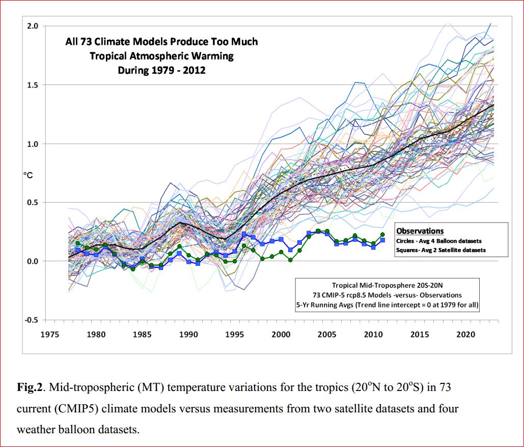
Fig.3 Comparison of Climate Models to Observations from the paper by R. Spencer et al. his Fig. 2 (reference to follow.)
In the above figure atmospheric temperature measurements made over a period of 32 years are plotted as data points on the graph. These temperature data were obtained from both satellite instruments and balloon borne instruments over the decades long timescales indicated in Fig.3.
Climate model predictions are also plotted in Fig. 3 as color coded solid curves. The black curve represents the running average of all 73 models.
If these climate models were any good, they would agree with temperature measurements shown in the data plot.
Instead of good agreement with the temperature data, what we see is long term systematic divergence of all 73 climate models from the data.
Notice all models predict substantial global warming (consensus of models!) while no models agree with the real climate data. Recall that models that disagree with new data in a systematic fashion are thereby proved to be invalid.
Because the models are so bad, the obvious systematic divergences with real data can readily be seen by even the most casual inspection of Fig.3.
It's clear that all 73 climate models in the figure have been invalidated by real world temperature measurements.
Further, we can observe that the divergence-from-new-data of the above plotted climate models is in agreement with our prediction that non-causal climate models must inevitably diverge from new data. That is, climate models such as these must fail upon extrapolation into the future.
(Why are there so many distinct climate models? Hint: Such models are termed semi-empirical models. Semi-empirical models contain many adjustable parameters, aka fudge factors.)
We can summarize the predictive performance of climate models by box scores below. A model scores 1 point in the event it demonstrates significant long term agreement with the corresponding new climate data sets.
How are climate models doing?
Here are the box scores:
Of course, models can be tweeked, modified or otherwise fixed up after they fail. When modelers do this in a way that agrees with the latest data, we have a new model. After such ad hoc fixes, the new models are considered invalid until they demonstrate significant long term agreement with new data, without further tweeking.
More on proxy time:
The parameter representing time, the time variable, does not appear in the physical theory of thermodynamics. One has thermodynamic state variables, but no time variable. Further, many climate simulation models do not support a time variable at all. For example, steady state flow models of the earth's ocean and atmosphere solve a set of equilibrium equations (with boundary) that do not have time as a variable.
How can such models having no time variable, be used to predict the future time evolution of the system?
Many such models make use of an artificial time or proxy time. Some quantity that varies monotonically with time, is used as a substitute for the time variable.
For, example, during time periods where atmospheric CO2 concentration is increasing steadily (monotonically) with time, one can plot model output as a function of CO2 concentration. Some modelers convert the independent variable from CO2 concentration to a proxy time variable in order to plot the model output as a function of proxy time.
What are non-causal models good for?
Paradoxically, non-causal models can be very useful for near term and periodic predictions. Non-causal predictive weather models are examples short term, day-to-day, and seasonal periodic forecasting. Successful Non-causal Models Exist and are Especially Useful for Describing Periodic Phenomena.
Interestingly some non-causal models can exhibit excellent long term predictive capabilities in a restricted range of model parameters for simple systems. For example, Newtonian gravitational field theory coupled with classical Newtonian mechanics is a non-causal model.
Why do we say Newtonian gravity is non-causal?
The Newtonian gravitational field equations are non-causal because they exhibit instantaneous action at a distance. There are no gravitational waves or propagation speeds for changes in the Newtonian gravitational field. General relativity on the other hand, does exhibit causality, there is no "action a a distance" in general relativity. Changes in the metric propagate at the speed of light in general relativity.
SIDEBAR
(Note for experts: Small amplitude spacetime metric perturbations described by the General Relativistic gravitational wave equations propagate at c. Some exotic processes such as inflation or various non-linear large amplitude perturbations can make the spacetime metric change much faster).
Back to Newtonian Mechanics...
Further, Newtonian mechanics does not obey the rules of special relativity. Despite these problems, Newtonian mechanics can work quite well as a predictive theory.
For simple systems, e.g. planetary orbits and the like, standard Newtonian gravity and mechanics have excellent predictive capabilities and often show impressive long term agreement with measured motions of planets, asteroids, some comets, slow speed space ships, etc. In many cases, the agreement with new measurements (data) extends over many years and many orbital periods. Importantly, periodic or quasi-periodic phenomena are often well described by non-causal models.
But Newtonian mechanics does not always work. The theory is contraindicated by measurements of time evolution of the perihelion of the planet Mercury. Further, Newtonian mechanics does not work for objects having velocities approaching the speed of light. Nor does Newtonian mechanics predict the observed deflection of light by massive objects (gravitational lens effect.) Enough on Newtonian mechanics for now.
What about Southern Hemisphere Sea Ice Data?
Fig. 2 Southern Hemisphere Sea Ice Area, Seasonal Variation by Year.
This data from agencies NOAA, NSIDC, and University of Bremen. Original data plot from this site: http://arctic.atmos.uiuc.edu/cryosphere/arctic.sea.ice.interactive.html
Briefly, the extensive data in this composite plot shows seasonal variations in southern hemisphere sea ice extent over 34 years from 1979 through 2013. We observe that record high sea ice extent occurred in 2013 yellow curve, and in 2012, red curve.
Of course, climate change is inevitable, but a 34 year data set is a rather small time period compared to the historic time scales of climate changes which occur on time scales of multi-decades, centuries, and millennia. The data presented in Fig. 2 indicate a rather stable climate over the timescales available so far.
Back to climate models...
Climate models used and misused to predict the future are more accurately termed climate forecasting models. Climate forecasting models get no credit for predicting the past.
Now let's examine the predictions of 73 (!) current climate forecasting models, and then compare them to real temperature data obtained for the years 1979 through 2012.
Fig.3 Comparison of Climate Models to Observations from the paper by R. Spencer et al. his Fig. 2 (reference to follow.)
What quantities are plotted in the graph shown in Fig. 3?
In the above figure atmospheric temperature measurements made over a period of 32 years are plotted as data points on the graph. These temperature data were obtained from both satellite instruments and balloon borne instruments over the decades long timescales indicated in Fig.3.
Climate model predictions are also plotted in Fig. 3 as color coded solid curves. The black curve represents the running average of all 73 models.
If these climate models were any good, they would agree with temperature measurements shown in the data plot.
Instead of good agreement with the temperature data, what we see is long term systematic divergence of all 73 climate models from the data.
Observations and Conclusions Fig. 3
Notice all models predict substantial global warming (consensus of models!) while no models agree with the real climate data. Recall that models that disagree with new data in a systematic fashion are thereby proved to be invalid.
Because the models are so bad, the obvious systematic divergences with real data can readily be seen by even the most casual inspection of Fig.3.
It's clear that all 73 climate models in the figure have been invalidated by real world temperature measurements.
Further, we can observe that the divergence-from-new-data of the above plotted climate models is in agreement with our prediction that non-causal climate models must inevitably diverge from new data. That is, climate models such as these must fail upon extrapolation into the future.
(Why are there so many distinct climate models? Hint: Such models are termed semi-empirical models. Semi-empirical models contain many adjustable parameters, aka fudge factors.)
We can summarize the predictive performance of climate models by box scores below. A model scores 1 point in the event it demonstrates significant long term agreement with the corresponding new climate data sets.
How are climate models doing?
Here are the box scores:
Earth's Real Climate
vs.
Climate Models
BOX SCORE 2013
vs.
Climate Models
BOX SCORE 2013
Earth's Climate: 73
Climate Model Predictions: 0
Extravagant claims of accuracy
vs.
Inevitable failure of extrapolation
BOX SCORE 2013
IPCC climate model extrapolation accuracy: 0
Synthetic Information prediction of failure: 1
We will add further examples of failure of climate models on extrapolation as time permits.
What about modeling of much simpler systems?
How's that going?
We observe that the US National Ignition Facility (NIF) at Lawrence Livermore Labs in California was extensively modeled by fluid codes that are much more sophisticated and accurate at what they do, than are climate models.What is NIF?
The NIF generates 192 powerful laser beams of UV light that are used to compress fusion targets aka pellets and heat fusion fuel in the target so as to achieve ignition of nuclear fusion reactions. Fluid modeling codes were used to predict the performance of the NIF.
Those state of the art fluid code models were used to validate the design of the NIF, and predicted that the NIF should achieve ignition of a nuclear fusion reaction in carefully designed targets containing fusion fuel.
The NIF was constructed and put into operation a few years ago. After a year long campaign of experiments in 2012 scientists found that NIF targets did not reach ignition conditions in the lab.
Box Score:
Nature 1
Models 0
The NIF is a fantastic scientific instrument for studying matter at extreme conditions of pressure and temperature. The scientific value of NIF is extraordinary.
We might say that the most important science from NIF so far was the invalidation of the fluid models. Such knowledge gained by rigorous testing of model predictions by means of precise experiments is central to scientific progress.
UPDATE ON NIF: FEB 12, 2014
Lawrence Livermore NIF team announces achievement of fusion energy gain greater than unity using a redesigned laser pulse strategy.
Congratulations to the NIF team.
Citation: http://dx.doi.org/10.1038/nature13008
"Energy gain greater than unity" means fusion energy generated by the laser driven implosion of the target is greater than the energy deposited in the fusion target by the laser beam pulse. An important milestone has been reached in the quest for fusion ignition.
However, energy gain of unity is not fusion ignition. Ignition would require a much larger energy gain, and that has not been achieved yet by NIF.
Roughly speaking, ignition means that after an initiating laser pulse, the fusion fuel would continue to generate fusion energy (to burn) in a self-sustaining nuclear fusion reaction. Like a miniature sun, the fusion target would continue to shine on its own, until its fuel is exhausted.
The Earth's climate system is a much more complex and challenging problem for fluid code modelers than is the NIF. It will take many decades of advances in the state-of-the-art of climate modeling to approach the accuracy of the Livermore fluid codes. Until a long track record of correct predictions of the actual future behavior of the Earth's climate is demonstrated by climate models, the models cannot be considered ready for prime-time.
SIDE BAR
_________________________________________
What's the Greenhouse Effect?
Attributed to early writings of astronomer Carl Sagan, the Greenhouse effect refers to absorption of "heat radiation" by atmospheric gases of a planet e.g Venus.
What is Heat Radiation?
Heat radiation is electromagnetic radiation (light waves) emitted by any warm substance as a consequence of thermodynamics. It's the reason hot steel glows in red, orange, yellow colors when heated in a blacksmith's forge, and the reason the Sun is yellow in color. Heat radiation can be viewed as a gas of photons having a temperature comparable to the temperature of the surrounding material surfaces.
The wavelength spectrum of heat radiation in a vacuum enclosure is well described by the Planck radiation theory which predicts a continuous wavelength spectrum given mathematically by the Planck Radiation Formula.
If the heat radiation is emitted into a gaseous material, the gas molecules will interact with the electromagnetic waves and may selectively absorb electromagnetic waves of certain wavelengths. A broad wavelength spectrum of electromagnetic radiation passing through a gas will therefore be attenuated in certain wavelength ranges called "absorption bands."
....to be continued. (2/18/2014)
SIDE BAR
______________________________________
Q: Is there a trend toward lower or higher minimum sea ice coverage in the time series data plotted in Fig. 1? Or, no significant trend either way?
Here we do a quickie trend analysis of the data in Fig. 1. Observe that the time series only has nine years. This kind of simple analysis is appropriate for small time series data sets. Of course, there are many many statistical analysis methods available, but with only a nine point sample, it's appropriate to use a simple and easy to follow method.
One way to get at the above question is simply to order the years 2005- 2013 from least to greatest sea ice coverage in mid-September. (We chose mid-September for this analysis because northern hemisphere sea ice reaches its annual minimum in the month of September. One could repeat the analysis below for other dates as well.)
If there is a trend toward lower sea ice coverage year to year, the next year in time sequence would be more likely to have lower sea ice. However, if it's equally likely to get higher or lower ice coverage in the next year, then there's no trend toward lower sea ice coverage.
So the question becomes, is the next year, after any given year, more likely to have lower sea ice coverage?
For example, if there was a steady (monotonic) decrease in mid-September sea ice area from 2005 through 2013, (as predicted by global warming climate models) then the lowest mid-September coverage would have occurred in 2013. Every previous year would have higher mid-September sea ice area, and 2005 would have the highest mid-September sea ice area out of the set of all years in the sample.
Now we can analyze the data in Fig. 1, and see what we get.
Note: We use the original higher resolution figure on the DMI website to read off sea ice area for each year in mid-September. Then we order years by relative minimum sea ice coverage in mid-September. That is, the lowest mid-September minimum occurred in 2012, the next lowest in 2007, and so on, for each year 2005 through 2013.
Here's our data collected from Fig. 1:
Lowest mid-September sea ice area occurred in 2012, blue curve; next lowest 2007, light blue curve; next lowest 2008, magenta; next lowest 2011, yellow; next lowest 2010, orange; next lowest 2009, baby blue or cyan; next lowest 2013, black, next lowest 2005, red, and highest sea ice coverage in mid-September occurred in 2006, green curve.
Conclusion:
That is, there is no systematic, year-to-year downward or upward trend, in northern hemisphere mid-September sea ice coverage, for the years for which we have mid-September data, 2005 through 2013.
One can see why this is so by examining year-to-year, increases or decreases in mid-September sea ice area in our data set above:
From 2005 to 2006 the ice area increased, from 2006 to 2007 ice area decreased, from 2007 to 2008 ice area increased, from 2008 to 2009 ice area increased, from 2009 to 2010 ice area decreased, from 2010 to 2011 ice area decreased, from 2011 to 2012 ice area decreased, from 2012 to 2013 ice area increased. We have four cases of increasing ice area and four cases of decreasing ice area over the period 2005 through 2013. Hence no trend of increase or decrease in mid-September sea ice area over the period 2005-2013.
Of course, there are many ways to analyze the data in Fig. 1. The above analysis gives a good indication of the existence or non-existence of a trend in a simple, easy to understand way. The above ordering of years by mid-September sea ice coverage area shows no systematic downward or upward trend.
(TO DO: some graphics to show the lack of a significant trend)
END SIDE BAR ______________________________________
"In science and elsewhere, we support freedom of inquiry, rational skepticism, and do not assume the conclusion."
- The Management